Wolfram Mathematica for Economists - Cobb Douglas Production Function
May 16, 2015
Mathematica is a very powerful and expressive programming language, which I use on a daily basis to do my research. It is unrivalled in Symbolic computation and it is very fast to test ideas, sketch a simple model or review results in journals. Once you see how powerful this tool is for note taking in maths heavy classes you will appreciate it too. However, before we dive into some interesting applications of Mathematica, let’s get acquainted with he basics.
First Things First
Before we start with some economics examples to get acquainted with Mathematica we need to understand the most important parts of the language and how they tie together. We look at how to evaluate expressions and then look at the most important types (i.e. integers, lists). After this me move on to learn how to defined and use basic functions.
How to evaluate a function
I assume that you have a working copy of Mathematica and know how to open and edit a notebook.
To evaluate a cell/input, press the combinations Shift+Enter while you have highlighted the cell you want to evaluate. It is customary to start programming in any language with a Hello World example. And here it is.
In[2]:=	Print["Hello World!"]
Out[2]=	Hello World!
Numbers
Let’s look at Integers first. To evaluate the 1+1 press Shift and Enter and you should get 2.
In[1]:=	1 + 1
Out[2]=	2
Mathematica avoids conversion of types to more general types whenever possible to avoid any loss of precision (i.e. 1/3 is not transformed from a rational to a real number since this would reduce precision). However if you need a real valued number you can coerce it to a Real by either doing an operation with a Real or explicitly transform it using the N function.
In[1]:=	1 + 1/2
Out[1]=	3/2
In[2]:=	1 + 0.5
Out[2]=	1.5
In[3]:=	N[3/2]
Out[3]=	1.5
The basic binary operators such as + , -, * and / are used just as you use them in any other context, no brackets, braces or other programming syntax is involved. However if you want to call a function which is not one of these you will need to call them using function syntax. By function syntax I mean to call for example \(\ln(x)\) which takes one argument using the Mathematica function Log[x].
In[1]:=	Log[1]
Out[1]=	0
Some things to note here. Official Mathematica functions start with a capital letter and are complete words in the CammelCase style, unlike MATLAB where functions are lower case and excessively shortened. Furthermore unlike MATLAB, Python, R, C/C++ and many other languages the arguments passed to a function are enclosed in square brackets [ ]. Parenthesis ( ) are used exclusively for grouping and define the order of operations.
Lists
Vectors, as you might already know, are simply Lists and in Mathematica vectors are effectively called List. Conversly a matrix is a vector of vectors and as such matrices are implemented in Mathematica as lists of lists. And higher order structures, say an array with 3 dimensions is a list of lists of lists. I guess you get the point. A list is a set of Expressions in curly braces {x1,x2,...,xn}. Since it is conceptually equal to a vector in linear algebra you can do the basic operations directly on them.
In[1]:=	{1, 2, 3} + {1, 2, 3}
Out[1]=	{2, 4, 6}
In[2]:=	2*{1,2,3}
Out[2]=	{2,4,6}
In[3]:=	{1, 2, 3}.{1, 2, 3}
Out[3]=	14
Lists are a central part of Mathematica and a lot of function parameters are supplied as lists.
Functions
One of the most widely used functional Production Functions is Cobb-Douglas \eqref{eq:1}. Lets look at this omnipresent function.
\begin{equation} Y=F(L,K)=A L^\alpha K^\beta \label{eq:1} \end{equation}
Usually in textbook examples it is assumed that the returns to scale are constant. This means effectively that \(\beta=1-\alpha\) and both are positive. Let’s now define this function in Mathematica. A function in mathematica takes the following form:
FuncName[var1_,var2_]:= functionBody
Here FuncName is the name you assign to the function, then in the square brackets we name the arguments here var1 and and var2. Note the underscore after the variable name. This underscore is necessary as it tells Mathematica “I want to take this and only this argument found here and name it var” 1 . For now just remember that every argument on the lhs of the definition must be defined with an underscore (_) after the name and can then be used in the rhs without the underscore. Then we have the := which effectively means “take the variables on the left and do something on the right”, unlike = the := operator tells Mathematica to not remember the rhs as is, but to evaluate it every time it is called. Here we define our function.
In[1]:=	CobbDouglas[L_,K_,A_,a_,b_]:=   A * L^a * K^b
In[2]:=	CobbDouglas[L_,K_,A_,a_]:= CobbDouglas[L,K,A,a,1-a]
A lot happened here, so lets look at what we just wrote. We defined a function called CobbDouglas on line 1. This function takes 5 arguments and assigns them to the rhs to compute a value. As you can see we have here both a and b which corresponds to the general case of a cobb douglas. On line 2 we define the special constant returns to scale variant. Note that we use the same function name CobbDouglas however with only 4 arguments. You can see on the right hand side this is nothing more than to say that if CobbDouglas is called with only 4 arguments we assume that we deal with a constant returns to scale situation. We have given the same name to two different functions varying only on the number (and possibly type) or arguments. Overloading as it is called is a way to define a function which behaves differently depending on what parameters it obtains.
Plot (3D)
Now lets move to a more fun application of this function.
Let’s plot the surface of our CobbDouglas function for all \(L\) and \(K\) from 0 to 1, holding \(A\) and \(\alpha\) fixed at 1 and 0.5 respectively.
We use the build-in Plot3D function to do this.
Plot3D[ CobbDouglas[l, k, 1, .5], {l, 0, 1}, {k, 0, 1},
    AxesLabel -> {"L","K","Y"},
    ColorFunction -> "DarkRainbow",
    MeshFunctions -> {#3 &}]
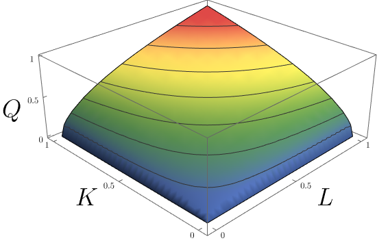
Now let’s look at this plot. We have told Plot3D to plot the CobbDouglas function for l from 0 to 1 passing this as a list, where the first element is the variable to which this interval applies. And we do the same thing for k. It is also good practice to label the axes and we do that by passing to the Plot3D option AxesLabel the list of labels to be used {"L","K","Y"}. Next we choose a nice ColorFunction. This function applies a predefined colour scale to our \(Y\) values. And finally, as good economists we plot some isoquants (i.e. level curves). Since isoquants are simply the combination of input factors which yield the same output \(Y\), we can tell Plot3D to place lines (i.e. Mesh) at constant values of \(Y\) by passing to the option MeshFunctions the pure function {#3 &}. I will cover pure functions in one of the next posts on Functional Programming.
Conclusion
Mathematica has a large community of users writing packages and offering advice on how to solve problems. The best such site is mathematica.stackexchange.com. If you have a question it has most likely been answered here. And last but not least Mathematica’s documentation online and offline is superb. Wolfram Mathematica has one of the best documentation I have come across complete of references, neat examples, possible applications and issues.
Remember: The Documentation is your Friend!
-
The underscore is part of Mathematica’s internal pattern matching. The pattern matching is very powerful approach when defining more complex functions. Take a look at the manual page ↩︎